An Sweave Demo
This is a demo for using the Sweave (via its wrapper Textile) command in R. To get started make a regular textile file (like this one) but give it the suffix .Rnw instead of .textile and then turn it into a textile file (foo.tex) with the R command:
Textile('foo.Rnw')So now we have a more complicated file chain:
foo.Rnw >> Textile >> foo.textile >> jekyll >> foo.html >> firefox
and what have we accomplished other than making it twice as annoying to the WYSIWYG crowd (having to run both Textile and jekyll to get anything that looks like the document)?
Well, we can now include R in our document. Here’s a simple example
> 2 + 2
[1] 4
What I actually typed in foo.Rnw was
 <<two>>=
 2 + 2
 @
This is not textile. It is a ``code chunk’’ to be processed by Sweave. When Sweave hits such a thing, it processes it, runs R to get the results, and stuffs (by default) the output in the textile file it is creating. The textile between code chunks is copied verbatim (except for Sexpr, about which see below). Hence to create a Rnw document you just write plain old textile interspersed with ``code chunks’’ which are plain old R.
Plots get a little more complicated. First we make something to plot (simulate regression data).
> n <- 50
> x <- seq(1, n)
> a.true <- 3
> b.true <- 1.5
> y.true <- a.true + b.true * x
> s.true <- 17.3
> y <- y.true + s.true * rnorm(n)
> out1 <- lm(y ~ x)
> summary(out1)
Call:
lm(formula = y ~ x)

Residuals:
     Min       1Q   Median       3Q      Max
-34.2291 -14.2846   0.7975  18.3229  33.8871

Coefficients:
            Estimate Std. Error t value Pr(>|t|)
(Intercept)   1.9520     5.5914   0.349    0.729
x             1.4033     0.1908   7.353 2.12e-09 ***
---
Signif. codes:  0 ‘***’ 0.001 ‘**’ 0.01 ‘*’ 0.05 ‘.’ 0.1 ‘ ’ 1

Residual standard error: 19.47 on 48 degrees of freedom
Multiple R-squared: 0.5298,	Adjusted R-squared:  0.52
F-statistic: 54.07 on 1 and 48 DF,  p-value: 2.116e-09
(for once we won’t show the code chunk itself, look at foo.Rnw if you want to see what the actual code chunk was).
The figure is produced by the following code
> plot(x, y)
> abline(out1)
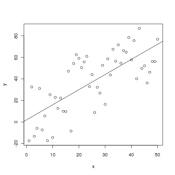
Note that x, y, and out1 are remembered from the preceding code chunk. We don’t have to regenerate them. All code chunks are part of one R ``session’’.
Now this was a little tricky. We did this with two code chunks, one visible and one invisible. First we did
 <<label=fig1plot,include=FALSE>>=
 plot(x, y)
 abline(out1)
 @
where the include=FALSE indicates that the output (text and graphics) should not go here (they will be some place else) and the label=fig1plot gives the code chunk a name (to be used later). And ``later’’ is almost immediate. Next we did
 <<label=fig1,fig=TRUE,echo=FALSE>>=
 <<fig1plot>>
 @
In this code chunk the fig=TRUE indicates that the chunk generates a figure. Sweave automagically makes both JPG and PDF files for the figure and automagically generates an appropriate !figname.jpg! command to include the plot. The echo=FALSE in the code chunk means just what it says (we’ve already seen the code — it was produced by the preceding chunk — and we don’t want to see it again, especially not in our figure). The <<fig1plot>> is an example of ``code chunk reuse’’. It means that we reuse the code of the code chunk named fig1plot. It is important that we observe the DRY/SPOT rule (don’t repeat yourself or single point of truth) and only have one bit of code for generating the plot. What the reader sees is guaranteed to be the code that made the plot. If we had used cut-and-paste, just repeating the code, the duplicated code might get out of sync after edits. The rest of this should be recognizable to anyone who has ever done a textile figure.
So making a figure is a bit more complicated in some ways but much simpler in others. Note the following virtues
- The figure is guaranteed to be the one described by the text (at least by the R in the text).
- No messing around with sizing or rotations. It just works!
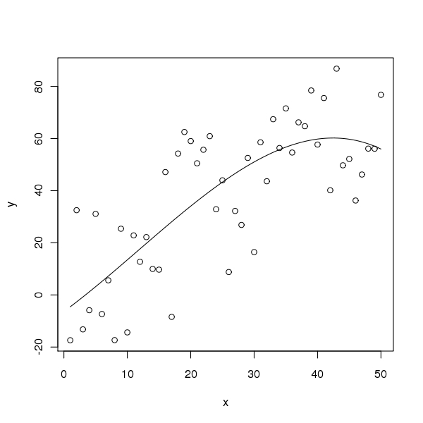
Note that if you don’t care to show the R code to make the figure, it is simpler still. Another figure shows another plot. What I actually typed in foo.Rnw was
 <<label=fig2,fig=TRUE,echo=FALSE>>=
 out3 <- lm(y ~ x + I(x^2) + I(x^3))
 plot(x, y)
 curve(predict(out3, newdata=data.frame(x=x)), add = TRUE)
 @
Now we just included the code for the plot in the figure (with echo=FALSE so it doesn’t show).
Also note that every time we rerun Sweave, figures change, the latter conspicuously (because the simulated data are random). Everything just works. This should tell you the main virtue of Sweave. It’s always correct. There is never a problem with stale cut-and-paste.
Simple numbers can be plugged into the text with the \Sexpr command, for example, the quadratic and cubic regression coefficients in the preceding regression were beta 2 = 0.0264 and beta 3 = -0.0007. Just magic! What I actually typed in foo.Rnw was
in the preceding regression were beta ~2~ = 0.0264 and beta ~3~ = -0.0007.The ascii command is used to make tables. (The following is the Sweave of another code chunk that we don’t explicitly show. Look at foo.Rnw for details.)
> out2 <- lm(y ~ x + I(x^2))
> foo <- anova(out1, out2, out3)
> foo
Analysis of Variance Table

Model 1: y ~ x
Model 2: y ~ x + I(x^2)
Model 3: y ~ x + I(x^2) + I(x^3)
  Res.Df   RSS Df Sum of Sq      F  Pr(>F)
1     48 18201
2     47 16571  1   1630.25 4.5680 0.03792 *
3     46 16417  1    154.21 0.4321 0.51424
---
Signif. codes:  0 ‘***’ 0.001 ‘**’ 0.01 ‘*’ 0.05 ‘.’ 0.1 ‘ ’ 1
> class(foo)
[1] "anova"      "data.frame"
So now we are ready to turn the matrix foo into a table.
ANOVA Table
| . Res.Df | RSS | Df | Sum of Sq | F | Pr(>F) |
|---|---|---|---|---|---|
| 48.00 | 18201.08 | ||||
| 47.00 | 16570.83 | 1.00 | 1630.25 | 4.57 | 0.04 |
| 46.00 | 16416.63 | 1.00 | 154.21 | 0.43 | 0.51 |
using the R chunk
 <<label=tab1,echo=FALSE,results=ascii>>=
 print(ascii(foo, caption = "ANOVA Table", include.rownames = FALSE), "textile")
 @
To summarize, Sweave is terrific, so important that soon we’ll not be able to get along without it. It’s virtues are
- The numbers and graphics you report are actually what they are claimed to be.
- Your analysis is reproducible. Even years later, when you’ve completely forgotten what you did, the whole write-up, every single number or pixel in a plot is reproducible.
- Your analysis actually works—-at least in this particular instance. The code you show actually executes without error.
- Toward the end of your work, with the write-up almost done you discover an error. Months of rework to do? No! Just fix the error and rerun
Sweaveandjekyll. One single problem like this and you will have all the time invested inSweaverepaid. - This methodology provides discipline. There’s nothing that will make you clean up your code like the prospect of actually revealing it to the world.
Whether we’re talking about homework, a consulting report, a textbook, or a research paper. If they involve computing and statistics, this is the way to do it.